Wednesday, April 8, 2015

Random Surface Roughness Generation using MATLAB program

Visit http://CivilEngineeringBible.com for newer posts and files
Today, I developed a MATLAB function to generate a random surface roughness for future study of a thermomechanical rough contact in Abaqus. here are results for different values of Ra and Rq (Roughness amplitude parameters):


For initial mesh Abaqus is used, for random generation of surface roughness MATLAB is used and for post processing Tecplot is used. if you need any further information feel free to contact me via my email address: Hosseinali.sut@gmail.com

Wednesday, March 25, 2015

3D elastic Finite Element MATLAB code + Abaqus Verification

Visit http://CivilEngineeringBible.com for newer posts and files
I wrote a finite element code for three-dimensional analysis of elastic body using MATLAB programming language.
Here is a video of the results + its verification with Abaqus:


Output results are shown in Tecplot; hexahedron elements are used; Basic conjugate gradient method (BCG) is used to solve linear solutions to be able to solve large number of nodes and elements.
Contact me via email (hosseinali.sut@gmail.com) for MATLAB files (functions):
main.m
basicconjugategradientsolution.m
B.m
rNrkb.m

2D elastic Finite Element MATLAB code + Abaqus Verification

Visit http://CivilEngineeringBible.com for newer posts and files
I wrote a finite element code (FEM Program) for two-dimensional analysis of elastic body using MATLAB programming language.
Here is a video of the results + its verification with Abaqus:


4-node elements ,4 Gauss points for numerical integration are used;.

Contact me via email (hosseinali.sut@gmail.com) for MATLAB files (functions).

*** Here is a solve example using both Abaqus and Code:
Normal Stress in X-direction, Abaqus result:


Normal Stress in X-direction, Code result:


Shear Stress in XY-direction, Abaqus result:


Shear Stress in XY-direction, Code result:


Normal Stress in Y-direction, Abaqus result:


Normal Stress in Y-direction, Code result:

Liver Mesh file

Visit http://CivilEngineeringBible.com for newer posts and files
Here is a liver mesh with tetrahedron elements that I generated.


Contact me via email (hosseinali.sut@gmail.com) for liver mesh files (nodes + elements).

3D Large Deformation Finite Element Analysis using MATLAB Code

Visit http://CivilEngineeringBible.com for newer posts and files
Here is the MATLAB code for 3D FEM analysis of a large deformation problem.


Both Total and Updated Lagrangian Descriptions are programmed; Tetrahedron elements are used.
Do not hesitate to contact me via email (hosseinali.sut@gmail.com) for MATLAB files:
main.m
At.m
BL.m
Gtensor.m
Volume.m

Finite Element Analysis of a Contact Problem using MATLAB Code

Visit http://CivilEngineeringBible.com for newer posts and files
Here is the results of my FEM MATLAB code for large deformation contact problem:
Both Penalty and Lagrange Multiplier methods are programmed.


Do not hesitate to contact me via email (hosseinali.sut@gmail.com) for MATLAB files:
At.m
Bbar.m
BL.m
FX.m
GreenSt.m
Gvector.m
J.m
main.m
MG.m
readdata.m
spk2c.m

FEM MATLAB code for Newmark 1D dynamic analysis of a 4 DOFs structure

Visit http://CivilEngineeringBible.com for newer posts and files
Here is the result of my MATLAB code for dynamic analysis of a four degrees of freedom structure:

Newmark method is used in this program.


Feel free to contact me via email (hosseinali.sut@gmail.com) for MATLAB files:
newmark_1d.m

Free download MATLAB file for Finite Element beam analysis using beam elements + solved examples

Visit http://CivilEngineeringBible.com for newer posts and files
Many structural systems used in practice consist of long slender members that are subjected to loading normal to their longitudinal axis and must resist bending and shear forces. They are called beams. Beams are governed by a fourth-order  differential equation.
beam element
Assumed degrees of freedom for a beam element used in this code.
Example1:
Consider a simple cantilever beam with a circular cross-section of 10 in diameter and a length of 400in. E = 30e6 psi. Load = 1000 lbs in downward direction at the right end of the beam.
Analytical solution for the mximum deflection and slope at the right end of the beam is as follows:
Slope = P(L^2)/2*EI =  0.0054
Deflection = P(L^3)/3*EI = 1.44866
and Finite Element result generated by MATLAB program is shown below:


Example2:
Consider a simply supported beam with a circular cross-section of 10 in diameter and a length of 400 in. The Young’s Modulus of the beam is 30e6. Load = 1000 lbs in downward direction at the right end of the beam.
Analytical solution -> Maximum deflection at the center of the beam is:
deflection = Ymax = P(L^3)/(48*EI) = 0.090541
slope = 0.0
and Finite Element results generated by MATLAB program for two element model and 4 element model are shown below:


Feel free to contact me via email (hosseinali.sut@gmail.com) for more details.
MATLAB Code is:
main.m *****************************
%%
% Developed by Massoud Hosseinali (hosseinali.sut@gmail.com) – 2015
% Finite element MATLAB program for beam analysis
%%
clear all;clc;close all;
Nodes = load(‘nodes.txt’); % coordinate of node
Elements = load(‘elements.txt’);    % first node, second node, E, I
numnode = length(Nodes); %Holds number of nodes
numelem = size(Elements,1); %Holds number of elements
K = zeros(2*numnode,2*numnode);
F = zeros(2*numnode, 1);
U = zeros(2*numnode, 1);
act = [ 2 3 4 5 6 7 8 10 ]; %Hold active DOFs
for ie = 1:numelem
DOFs = [2*Elements(ie, 1)-1, 2*Elements(ie, 1), 2*Elements(ie, 2)-1, 2*Elements(ie, 2)]; %Holds element’s DOFs
L = abs(Nodes(Elements(ie,2)) – Nodes(Elements(ie,1)));  %Holds length of element
E = Elements(ie,3); %Holds modolus of elasticiy of element
I = Elements(ie,4); %Holds moment of inertia of element
K(DOFs,DOFs) = K(DOFs,DOFs) + (E*I/(L^3))*[12 6*L -12 6*L; 6*L 4*L^2 -6*L 2*L^2; -12 -6*L 12 -6*L; 6*L 2*L^2 -6*L 4*L^2]; % Calculates the element stiffness matrix and assembles it to the global stiffness matrix
end
F(5) = -1000;
U(act) = K(act,act)\F(act); % Solves linear solutions
icounter= 0;
for ie = 1:numelem
DOFs = [2*Elements(ie, 1)-1, 2*Elements(ie, 1), 2*Elements(ie, 2)-1, 2*Elements(ie, 2)]; %Holds element’s DOFs
L = abs(Nodes(Elements(ie,2)) – Nodes(Elements(ie,1)));  %Holds length of element
for s = 0:(0.1*L):L
icounter = icounter  + 1;
slratio = s/L;
%Shape functions
N1 = (1-3*slratio^2+2*slratio^3);
N2 = L*(slratio-2*slratio^2+slratio^3);
N3 = (3*slratio^2-2*slratio^3);
N4 = L*(-slratio^2+slratio^3);
N = [N1 N2 N3 N4];
x(icounter) = s + Nodes(Elements(ie,1));
v(icounter) = N*U(DOFs);
end
end
hold all
plot(x,v);
plot(Nodes, U(1:2:end,1), ‘o’, ‘MarkerSize’, 10, ‘Color’, ‘Black’)
xlabel(‘X’)
ylabel(‘Deflection’)
grid on
Elements.txt (Sample) *******************
1 2 30e6 490.8739
2 3 30e6 490.8739
3 4 30e6 490.8739
4 5 30e6 490.8739
Nodes.txt (Sample) *******************
0
100
200
300
400

Free download MATLAB file for finite element analysis of plane trusses + solved example + visualization, including temperature changes and initial strains

Visit http://CivilEngineeringBible.com for newer posts and files
A truss is a structure in which members are arranged in such a way that they are subjected to axial loads only. The joints in trusses are considered pinned. Plane trusses, where all members are assumed to be in x-y plane, are considered in this MATLAB code.

Descriptions and notes:


Example:
Consider a simple six-bar pin-jointed structure shown below. All members have the same cross-sectional area and are of same material, E = 200 and A = 0.001; The load P = 20 and acts at an angle of 30 degrees.


each node has two degree of freedom and thus there are a total of ten degrees of freedom.
It is solved using this MATLAB code and the results are as follows:


# UPDATE 1: An amplification factor variable is added for better visualization. Moreover, MATLAB file plots initial and deformed configurations. An example plot is shown above.

# UPDATE 2: Displacement line (pink in figure) can be plotted now, figure below shows an example figure.


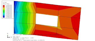
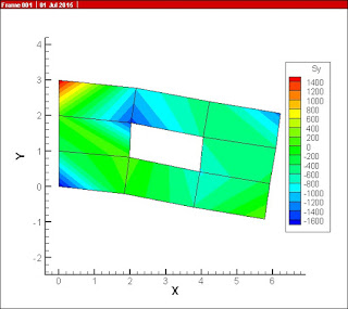
# UPDATE 3: Temperature change and initial strains are included in this update. Below is a solved example:
Consider the five-bar pin-jointed structure below:
All members have the same cross-sectional area and are of same material. The first element undergoes a temperature rise of 100 F. MATLAB code results are shown below:
Note that displacement amplification factor is 120.


For updated codes contact me (hosseinali.sut@gmail.com).

Easy Download:
http://www.4shared.com/rar/GGJIu4zZce/finite_element_matlab_files_fo.html
http://www.uploadbaz.com/p85s0gb1oe8x
http://s4.picofile.com/file/8179621476/finite_element_matlab_files_for_truss_analysis.rar.html


MATLAB files' content (without updates; free):
main.m **********************
%%
% Developed by Massoud Hosseinali (hosseinali.sut@gmail.com) – 2015
% Finite element MATLAB program for truss analysis
%%
clear all;clc;close all;
Nodes = load(‘nodes.txt’); %x, y coordinates
Elements = load(‘elements.txt’);    % first node, second node, E, A
numnode = length(Nodes); %Holds number of nodes
numelem = size(Elements,1); %Holds number of elements
K = zeros(2*numnode,2*numnode);
F = zeros(2*numnode, 1);
U = zeros(2*numnode, 1);
strain = zeros(numelem,1);
stress= zeros(numelem,1);
axialforce =zeros(numelem,1);
act = 1:2*numnode; %Holds active DOFs
act([1 2 5 6 7 8]) = [];
for ie = 1:numelem
DOFs = [2*Elements(ie, 1)-1, 2*Elements(ie, 1), 2*Elements(ie, 2)-1, 2*Elements(ie, 2)]; %Holds element’s DOFs
X1 = Nodes(Elements(ie,1), 1);
Y1 = Nodes(Elements(ie,1), 2);
X2 = Nodes(Elements(ie,2), 1);
Y2 = Nodes(Elements(ie,2), 2);
L = sqrt((X2-X1)^2+(Y2-Y1)^2); %Holds length of element
ms = (Y2-Y1)/L;ls=(X2-X1)/L;
E = Elements(ie,3); %Holds modolus of elasticiy of element
A = Elements(ie,4); %Holds cross sectional area of element
K(DOFs,DOFs) = K(DOFs,DOFs) + (E*A/L)*[ls^2 ls*ms -ls^2 -ls*ms; ls*ms ms^2 -ls*ms -ms^2; -ls^2 -ls*ms ls^2 ls*ms; -ls*ms -ms^2 ls*ms ms^2]; % Calculates the element stiffness matrix and assembles it to the global stiffness matrix
end
F(3) = 10000; F(4) = 10000*sqrt(3);
U(act) = K(act,act)\F(act);
for ie = 1:numelem
DOFs = [2*Elements(ie, 1)-1, 2*Elements(ie, 1), 2*Elements(ie, 2)-1, 2*Elements(ie, 2)]; %Holds element’s DOFs
X1 = Nodes(Elements(ie,1), 1);
Y1 = Nodes(Elements(ie,1), 2);
X2 = Nodes(Elements(ie,2), 1);
Y2 = Nodes(Elements(ie,2), 2);
L = sqrt((X2-X1)^2+(Y2-Y1)^2); %Holds length of element
ms = (Y2-Y1)/L;ls=(X2-X1)/L;
d = [ls ms 0 0; 0 0 ls ms]*U(DOFs);
strain(ie) = (d(2) – d(1))/L;
stress(ie)= Elements(ie, 3)*strain(ie);
axialforce(ie) = stress(ie)*Elements(ie,4);
end
Nodes.txt (example 1) ****************
0 0
4000 0
0 3000
4000 3000
2000 2000
Elements.txt (example 1) *************
1 2 200 1000
2 5 200 1000
5 3 200 1000
2 4 200 1000
1 5 200 1000
5 4 200 1000